Introduction to spatial data analysis with geopandas#
Now as we have learned how to create and represent geographic data in Python using shapely objects, we will continue and use geopandas [1] as our main tool for spatial data analysis. Geopandas extends the capacities of pandas (which we covered in the Part I of the book) with geospatial operations. The main data structures in geopandas are GeoSeries and GeoDataFrame which extend the capabilities of Series and DataFrames from pandas. This means that we can use many familiar methods from pandas also when working with geopandas and spatial features. A GeoDataFrame is basically a pandas.DataFrame that contains one column for geometries. The geometry column is a GeoSeries which contains the geometries as shapely objects (points, lines, polygons, multipolygons etc.).
Getting started with geopandas#
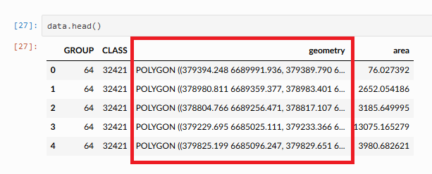
Figure 6.10. Geometry column in a GeoDataFrame.
Similar to importing import pandas as pd, we will import geopandas as gpd:
import geopandas as gpd
Reading a file#
In geopandas, we can use a generic function .from_file() for reading in various data formats. The data-folder contains some census data from Austin, Texas downloaded from the U.S Census bureau [2]. Let’s first define the path to the file.
from pathlib import Path

data_folder = Path("data/Austin")
fp = data_folder / "austin_pop_2019.gpkg"
print(fp)
data\Austin\austin_pop_2019.gpkg
Now we can pass this filepath to geopandas.
data = gpd.read_file(fp)
Let’s check the data type.
type(data)
geopandas.geodataframe.GeoDataFrame
Here we see that our data -variable is a GeoDataFrame which extends the functionalities of
DataFrame to handle spatial data. We can apply many familiar pandas methods to explore the contents of our GeoDataFrame. Let’s have a closer look at the first rows of the data.
data.head()
| pop2019 | tract | geometry | |
|---|---|---|---|
| 0 | 6070.0 | 002422 | POLYGON ((615643.487 3338728.496, 615645.477 3... |
| 1 | 2203.0 | 001751 | POLYGON ((618576.586 3359381.053, 618614.330 3... |
| 2 | 7419.0 | 002411 | POLYGON ((619200.163 3341784.654, 619270.849 3... |
| 3 | 4229.0 | 000401 | POLYGON ((621623.757 3350508.165, 621656.294 3... |
| 4 | 4589.0 | 002313 | POLYGON ((621630.247 3345130.744, 621717.926 3... |
Question 6.2#
Figure out the following information from our input data using your pandas skills:
Number of rows?
Number of census tracts (based on column
tract)?Total population (based on column
pop2019)?
# Solution

print("Number of rows", len(data))
print("Number of census tract", data["tract"].nunique())
print("Total population", data["pop2019"].sum())
Number of rows 130
Number of census tract 130
Total population 611935.0
It is always a good idea to explore your data also on a map. Creating a simple map from a GeoDataFrame is really easy. You can use the .plot() -function from geopandas that creates a map based on the geometries of the data. geopandas actually uses matplotlib for plotting which we introduced in Part 1 of this book. Let’s try it out, and do a quick visualization of our data.
data.plot()
<AxesSubplot: >
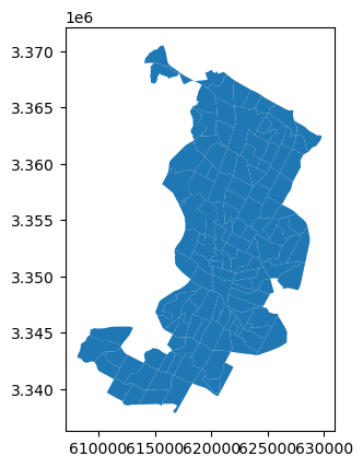
Figure 6.11. Census tract polygons for Austin, Texas, USA.
Voilá! Now we have a quick overview of the geometries in this data. The x and y axes in the plot are based on the coordiante values of the geometries.
Geometries in geopandas#
A GeoDataFrame has one column for storing geometries. By default, geopandas looks for the geometries from a column called geometry. It is also possible to define other columns as the geometry column. Th geometry column is a GeoSeries that contains shapely’s geometric objects. Let’s have a look at the geometry column of our sample data.
data["geometry"].head()
0    POLYGON ((615643.487 3338728.496, 615645.477 3...
1    POLYGON ((618576.586 3359381.053, 618614.330 3...
2    POLYGON ((619200.163 3341784.654, 619270.849 3...
3    POLYGON ((621623.757 3350508.165, 621656.294 3...
4    POLYGON ((621630.247 3345130.744, 621717.926 3...
Name: geometry, dtype: geometry
As we can see here, the geometry column contains polygon geometries. Since these polygons are shapely objects, it is possible to use shapely methods for handling them also in geopandas. Many of the methods can be applied all at once to the whole GeoDataFrame.
Let’s proceed to calculating area of the census tract polygons. At this point, it is good to note that the census data are in a metric coordinate reference system, so the area values will be given in square meters.
data["geometry"].area
0      4.029772e+06
1      1.532030e+06
2      3.960344e+06
3      2.181762e+06
4      2.431208e+06
           ...
125    2.321182e+06
126    4.388407e+06
127    1.702764e+06
128    3.540893e+06
129    2.054702e+06
Length: 130, dtype: float64
The same result can be achieved by using the syntax data.area. Let’s convert the area values from square meters to square kilometers and store them into a new column.
# Get area and convert from m2 to km2
data["area_km2"] = data.area / 1000000
Check the output.
data["area_km2"].head()
0    4.029772
1    1.532030
2    3.960344
3    2.181762
4    2.431208
Name: area_km2, dtype: float64
Question 6.3#
Using your pandas skills, create a new column pop_density_km2 and populate it with population density values (population / km2) calculated based on columns pop2019 and area_km2. Print out answers to the following questions:
What was the average population density in 2019?
What was the maximum population density per census tract?
# Solution

# Calculate population density
data["pop_density_km2"] = data["pop2019"] / data["area_km2"]

# Print out average and maximum values
print("Average:", round(data["pop_density_km2"].mean()), "pop/km2")

print("Maximum:", round(data["pop_density_km2"].max()), "pop/km2")
Average: 2397 pop/km2
Maximum: 11324 pop/km2
Writing data into a file#
It is possible to export spatial data into various data formats using the .to_file() method in geopandas. Let’s practice writing data into the geopackage file format. Before proceeding, let’s check how the data looks like at this point.
data.head()
| pop2019 | tract | geometry | area_km2 | pop_density_km2 | |
|---|---|---|---|---|---|
| 0 | 6070.0 | 002422 | POLYGON ((615643.487 3338728.496, 615645.477 3... | 4.029772 | 1506.288769 |
| 1 | 2203.0 | 001751 | POLYGON ((618576.586 3359381.053, 618614.330 3... | 1.532030 | 1437.961408 |
| 2 | 7419.0 | 002411 | POLYGON ((619200.163 3341784.654, 619270.849 3... | 3.960344 | 1873.322183 |
| 3 | 4229.0 | 000401 | POLYGON ((621623.757 3350508.165, 621656.294 3... | 2.181762 | 1938.341868 |
| 4 | 4589.0 | 002313 | POLYGON ((621630.247 3345130.744, 621717.926 3... | 2.431208 | 1887.538655 |
Write the data into a file using the .to_file() method.
# Create a output path for the data
output_fp = data_folder / "austin_pop_density_2019.gpkg"

# Write the file
data.to_file(output_fp)
Question 6.4#
Read the output file using geopandas and check that the data looks ok.
# Solution

temp = gpd.read_file(output_fp)

# Check first rows
temp.head()
| pop2019 | tract | area_km2 | pop_density_km2 | geometry | |
|---|---|---|---|---|---|
| 0 | 6070.0 | 002422 | 4.029772 | 1506.288769 | POLYGON ((615643.487 3338728.496, 615645.477 3... |
| 1 | 2203.0 | 001751 | 1.532030 | 1437.961408 | POLYGON ((618576.586 3359381.053, 618614.330 3... |
| 2 | 7419.0 | 002411 | 3.960344 | 1873.322183 | POLYGON ((619200.163 3341784.654, 619270.849 3... |
| 3 | 4229.0 | 000401 | 2.181762 | 1938.341868 | POLYGON ((621623.757 3350508.165, 621656.294 3... |
| 4 | 4589.0 | 002313 | 2.431208 | 1887.538655 | POLYGON ((621630.247 3345130.744, 621717.926 3... |
# Solution

# You can also plot the data for a visual check
temp.plot()
<AxesSubplot: >