Preparing GeoDataFrames from geographic data#

Reading data into Python is usually the first step of an analysis workflow. There are various different GIS data formats available such as Shapefile 1, GeoJSON 2, KML 3, and GeoPackage 4. Geopandas is capable of reading data from all of these formats (plus many more).

This tutorial will show some typical examples how to read (and write) data from different sources. The main point in this section is to demonstrate the basic syntax for reading and writing data using short code snippets. You can find the example data sets in the data-folder. However, most of the example databases do not exists, but you can use and modify the example syntax according to your own setup.

Reading vector data#

In geopandas, we can use a generic function .from_file() for reading in various vector data formats. When reading files with geopandas, the data are passed on to the fiona library under the hood for reading the data. This means that you can read and write all data formats supported by fiona with geopandas.

import geopandas as gpd
import fiona

Let’s check which drivers are supported by fiona.

fiona.supported_drivers

{'DXF': 'rw',
 'CSV': 'raw',
 'OpenFileGDB': 'raw',
 'ESRIJSON': 'r',
 'ESRI Shapefile': 'raw',
 'FlatGeobuf': 'raw',
 'GeoJSON': 'raw',
 'GeoJSONSeq': 'raw',
 'GPKG': 'raw',
 'GML': 'rw',
 'OGR_GMT': 'rw',
 'GPX': 'rw',
 'Idrisi': 'r',
 'MapInfo File': 'raw',
 'DGN': 'raw',
 'PCIDSK': 'raw',
 'OGR_PDS': 'r',
 'S57': 'r',
 'SQLite': 'raw',
 'TopoJSON': 'r'}

In the list of supported drivers, r is for file formats fiona can read, and w is for file formats it can write. Letter a marks formats for which fiona can append new data to existing files.

Let’s read in some sample data to see the basic syntax.

# Read Esri Shapefile
fp = "data/Austin/austin_pop_2019.shp"
data = gpd.read_file(fp)
data.head()

	fid	pop2019	tract	geometry
0	1.0	6070.0	002422	POLYGON ((615643.487 3338728.496, 615645.477 3...
1	2.0	2203.0	001751	POLYGON ((618576.586 3359381.053, 618614.330 3...
2	3.0	7419.0	002411	POLYGON ((619200.163 3341784.654, 619270.849 3...
3	4.0	4229.0	000401	POLYGON ((621623.757 3350508.165, 621656.294 3...
4	5.0	4589.0	002313	POLYGON ((621630.247 3345130.744, 621717.926 3...

The same syntax works for other commong vector data formats.

# Read file from Geopackage
fp = "data/Austin/austin_pop_2019.gpkg"
data = gpd.read_file(fp)

# Read file from GeoJSON
fp = "data/Austin/austin_pop_2019.geojson"
data = gpd.read_file(fp)

# Read file from MapInfo Tab
fp = "data/Austin/austin_pop_2019.tab"
data = gpd.read_file(fp)

Some file formats such as GeoPackage and File Geodatabase files may contain multiple layers with different names wihich can be speficied using the layer -parameter. Our example geopackage file has only one layer with the same name as the file, so we don’t actually need to specify it to read in the data.

# Read spesific layer from Geopackage
fp = "data/Austin/austin_pop_2019.gpkg"
data = gpd.read_file(fp, layer="austin_pop_2019")

# Read file from File Geodatabase
# fp = "data/Finland/finland.gdb"
# data = gpd.read_file(fp, driver="OpenFileGDB", layer="municipalities")

(write intro about enabling additional drivers and reading in the KML file)

# Enable KML driver
gpd.io.file.fiona.drvsupport.supported_drivers["KML"] = "rw"

# Read file from KML
fp = "data/Austin/austin_pop_2019.kml"
# data = gpd.read_file(fp)

Writing vector data#

We can save spatial data to various vector data formats using the .to_file() function in geopandas which also relies on fiona. It is possible to specify the output file format using the driver parameter, however, for most file formats it is not needed as the tool is able to infer the driver from the file extension.

# Write to Shapefile (just make a copy)
outfp = "data/temp/austin_pop_2019.shp"
data.to_file(outfp)

# Write to Geopackage (just make a copy)
outfp = "data/Temp/austin_pop_2019.gpkg"
data.to_file(outfp, driver="GPKG")

# Write to GeoJSON (just make a copy)
outfp = "data/Temp/austin_pop_2019.geojson"
data.to_file(outfp, driver="GeoJSON")

# Write to MapInfo Tab (just make a copy)
outfp = "data/Temp/austin_pop_2019.tab"
data.to_file(outfp)

# Write to same FileGDB (just add a new layer) - requires additional package installations(?)
# outfp = "data/finland.gdb"
# data.to_file(outfp, driver="FileGDB", layer="municipalities_copy")

# Write to KML (just make a copy)
outfp = "data/Temp/austin_pop_2019.kml"
# data.to_file(outfp, driver="KML")

Creating a GeoDataFrame from scratch#

It is possible to create spatial data from scratch by using shapely’s geometric objects and geopandas. This is useful as it makes it easy to convert, for example, a text file that contains coordinates into spatial data layers. Let’s first try creating a simple GeoDataFrame based on coordinate information that represents the outlines of the Senate square in Helsinki, Finland. Here are the coordinates based on which we can create a Polygon object using `shapely.

from shapely.geometry import Polygon

# Coordinates of the Helsinki Senate square in decimal degrees
coordinates = [
    (24.950899, 60.169158),
    (24.953492, 60.169158),
    (24.953510, 60.170104),
    (24.950958, 60.169990),
]

# Create a Shapely polygon from the coordinate-tuple list
poly = Polygon(coordinates)

Now we can use this polygon and geopandas to create a GeoDataFrame from scratch. The data can be passed in as a list-like object. In our case we will only have one row and one column of data. We can pass the polygon inside a list, and name the column as geometry so that geopandas will use the contents of that column the geometry column. Additionally, we could define the coordinate reference system for the data, but we will skip this step for now. For details of the syntax, see documentation for the DataFrame constructor and GeoDataFrame constructor online.

newdata = gpd.GeoDataFrame(data=[poly], columns=["geometry"])

newdata

	geometry
0	POLYGON ((24.95090 60.16916, 24.95349 60.16916...

We can also add additional attribute information to a new column.

# Add a new column and insert data
newdata.at[0, "name"] = "Senate Square"

# Check the contents
newdata

	geometry	name
0	POLYGON ((24.95090 60.16916, 24.95349 60.16916...	Senate Square

There it is! Now we have two columns in our data; one representing the geometry and another with additional attribute information. From here, you could proceed into adding additional rows of data, or printing out the data to a file.

Creating a GeoDataFrame from a text file#

A common case is to have coordinates in a delimited textfile that needs to be converted into spatial data. We can make use of pandas, geopandas and shapely for doing this.

The example data contains point coordinates of airports derived from openflights.org 5. Let’s read in a couple of useful columns from the data for further processing.

import pandas as pd

airports = pd.read_csv(
    "data/Airports/airports.txt",
    usecols=["Airport ID", "Name", "City", "Country", "Latitude", "Longitude"],
)

airports.head()

	Airport ID	Name	City	Country	Latitude	Longitude
0	1	Goroka Airport	Goroka	Papua New Guinea	-6.081690	145.391998
1	2	Madang Airport	Madang	Papua New Guinea	-5.207080	145.789001
2	3	Mount Hagen Kagamuga Airport	Mount Hagen	Papua New Guinea	-5.826790	144.296005
3	4	Nadzab Airport	Nadzab	Papua New Guinea	-6.569803	146.725977
4	5	Port Moresby Jacksons International Airport	Port Moresby	Papua New Guinea	-9.443380	147.220001

len(airports)

There are over 7000 airports in the data and we can use the coordinate information available in the Latitude and Longitude columns for visualizing them on a map. The coordinates are stored as Decimal degrees, meaning that the appropriate coordinate reference system for these data is WGS 84 (EPSG:4326).

There is a handy tool in geopandas for generating an array of Pointobjects based on x and y coordinates called .points_from_xy(). The tool assumes that x coordinates represent longitude and that y coordinates represent latitude.

airports["geometry"] = gpd.points_from_xy(
    x=airports["Longitude"], y=airports["Latitude"], crs="EPSG:4326"
)

airports = gpd.GeoDataFrame(airports)
airports.head()

	Airport ID	Name	City	Country	Latitude	Longitude	geometry
0	1	Goroka Airport	Goroka	Papua New Guinea	-6.081690	145.391998	POINT (145.39200 -6.08169)
1	2	Madang Airport	Madang	Papua New Guinea	-5.207080	145.789001	POINT (145.78900 -5.20708)
2	3	Mount Hagen Kagamuga Airport	Mount Hagen	Papua New Guinea	-5.826790	144.296005	POINT (144.29601 -5.82679)
3	4	Nadzab Airport	Nadzab	Papua New Guinea	-6.569803	146.725977	POINT (146.72598 -6.56980)
4	5	Port Moresby Jacksons International Airport	Port Moresby	Papua New Guinea	-9.443380	147.220001	POINT (147.22000 -9.44338)

Now we have the point geometries as shapelyobjects in the geometry-column ready to be plotted on a map.

airports.plot(markersize=0.1)

<AxesSubplot: >

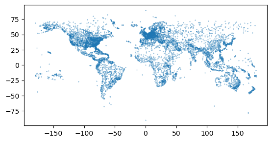
Figure 6.12. A basic plot showing the airports from openflights.org.

Footnotes#

1: https://en.wikipedia.org/wiki/Shapefile
2: https://en.wikipedia.org/wiki/GeoJSON
3: https://en.wikipedia.org/wiki/Keyhole_Markup_Language
4: https://en.wikipedia.org/wiki/GeoPackage
5: https://openflights.org/data.html

Preparing GeoDataFrames from geographic data

Contents