Retrieving OpenStreetMap data#
What is OpenStreetMap?#
OpenStreetMap [1] (OSM) is a free, editable map of the world that is created by a global community of mappers. OSM is often referred to as “the Wikipedia of maps” meaning that anyone can update the contents. When using OSM data, appropriate credit should be given to OpenStreetMap and its contributors (see OSM Copyright and License [2]).
OpenStreetMap data are increasingly used in various map-based applications and as input for geographic data analysis. In many regions, OSM is the best data available on streets, buildings and amenities, or at least the best data source that is openly available. While the map is never complete, many regions and especially urban areas are relatively well covered in OSM. Various organized mapping campaings exists to update OSM in areas that lack detailed map data (check out Humanitarian OpenStreetMap Team [3]).
OSM can be used as source data for various tasks such as routing and geocoding, and as bacground maps for visualizing analysis results. Relevant map feature categories include:
street networks
buildings
amenities
landuse
natural elements
boundaries
In OpenStreetMap, map features are labeled using tags consisting of a key that describes the category (such as “highway” or “building”) and a value that describes the type of object within the category (such as “motorway” or “aparments”). It is thus possible, for example, to fetch all available streets or limit the search only to specific types of streets. Information on various map features and their associated tags is fundamental for correctly querying the data.
Excerpts of OSM data are available to download from different sources, such as the Geofabrik Download Server [4]. Computationally, the Overpass API [5] can be used for querying and fetching parts of OSM data for further analysis.
A good way to start working with OSM data is to view the map from an area you are familiar with. The great thing about OSM is that anyone can sign up and make edits to the map. There are various discussion forums and mapping projects that support new (and old) mappers. The OSM wiki [6] provides an extensive overview for anyone planning to use or produce OSM data.
Question 9.1#
Go to www.openstreetmap.org and zoom the map to an area that you are familiar with.
Does the map look complete?
Are there any geometric features (roads, buildings, bus stops, service locations) missing?
Inspect further some of the features; are there any attribute information missing (street names, building addresses, service names or opening hours)?
You can check the intended tags for various map freatures from the OSM wiki [7]. If you spotted some missing information, freel free to create an OpenStreetMap account, log in, and update the map!
Downloading OpenStreetMap data with OSMnx#
Osmnx [8] is a Python package that makes it easy to download, model and analyze street networks and other geospatial features from OpenSteetMap (Boeing, 2024). Osmnx relies on geopandas and another module called networkx, which enables network analysis. For latest updates, installation instructions, and complete user reference, see osmnx documentation [9].
Osmnx uses the Overpass API for querying data from OSM. Map queries can be defined by city name, polygon, bounding box or an address or a point location and a buffer distance. There are different functions available to query data from the Overpass API using osmnx depending on the way in which the spatial location is defined. In addition, a set of tags can be specified to select which map features to download. Tags are passed to these functions as a dictionary allowing querying multiple tags at the same time.
Here, we will see how to fetch OSM data from a central area in downtown Helsinki. We will define our queries using a place name (“Kamppi, Helsinki, Finland”).
Defining the area of interest#
Let’s start by importing osmnx and getting the boundaries of our area of interest. Osmnx uses nominatim to geocode the place name. Notice that the place name needs to exists in OpenStreetMap, otherwise the query will fail.
import osmnx as ox

place = "Kamppi, Helsinki, Finland"
aoi = ox.geocoder.geocode_to_gdf(place)
aoi.explore()
Figure 9.1. Interactive map displaying the area of interest with a background map. Source: OpenStreetMap contributors.
Street network#
We can download street network data from our area of interest usign the osmnx graph module. The function downloads the street network data from OSM and construct a networkx graph model that can be used for routing.
graph = ox.graph.graph_from_place(place)
type(graph)
networkx.classes.multidigraph.MultiDiGraph
Let’s have a closer look a the street nework using an osmnx function that plots the graph:
# Plot the streets
fig, ax = ox.plot.plot_graph(graph, figsize=(6, 6))
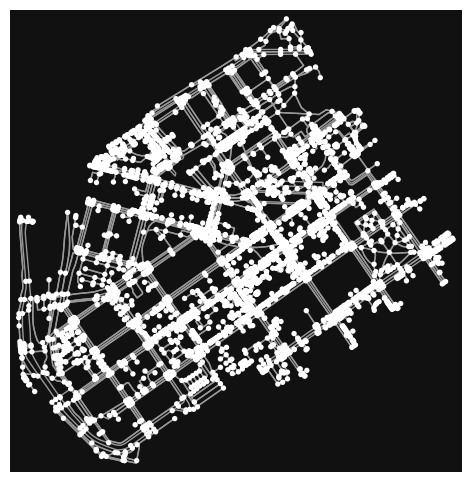
Figure 9.2. Graph edges and nodes.
From here we can see that our graph contains nodes (the points) and edges (the lines) of the network graph. There are various tools available in osmnx and networkx to continue modifying and analyzing this network graph. It would also be possible to limit the search to contain only specific street segments, such as all public streets or all streets and paths that cyclists or pedestrians can use. You can read more about working with street network graphs in the osmnx online documentation.
For now, we are only interested in the geometry and attributes of the street network and will convert the streets (edges of the network) into a GeoDataFrame using the osmnx function graph_to_gdfs().
edges = ox.convert.graph_to_gdfs(graph, nodes=False, edges=True)
edges.head(2)
| osmid | highway | lanes | maxspeed | name | oneway | reversed | length | geometry | junction | width | tunnel | access | service | bridge | |||
|---|---|---|---|---|---|---|---|---|---|---|---|---|---|---|---|---|---|
| u | v | key | |||||||||||||||
| 25216594 | 1372425721 | 0 | 23717777 | primary | 2 | 40 | Porkkalankatu | True | False | 10.403735 | LINESTRING (24.92106 60.16479, 24.92087 60.16479) | NaN | NaN | NaN | NaN | NaN | NaN |
| 1372425714 | 0 | 23856784 | primary | 2 | 40 | Mechelininkatu | True | False | 40.885163 | LINESTRING (24.92106 60.16479, 24.92095 60.164... | NaN | NaN | NaN | NaN | NaN | NaN |
Other map features#
Downloading building footprints, points of interests such as services and other map features is possible using the osmnx features module. As for street networks, map features can be queried based on varying spatial input (form bounding box, polygon, place name, or around a point or an address). Here, we will demonstrate the use of a place name search from our area of interest in Helsinki, Finland.
place = "Kamppi, Helsinki, Finland"
tags = {"building": True}

buildings = ox.features.features_from_place(place, tags)
This way, we get all map features that contain the building-tag regardless of its value. The downloaded OSM data comes with plenty of information representing various attributes of the features that OSM contributors have added. At the time of writing, the building data from central Helsinki contained 120 different columns.
len(buildings.columns)
120
You can see names of all available columns by running list(buildings.columns). Let’s check the contents of some of the available columns:
buildings[["building", "name", "addr:city", "geometry"]].head()
| building | name | addr:city | geometry | ||
|---|---|---|---|---|---|
| element | id | ||||
| node | 11711721042 | yes | Nice Bike Pyörähuolto | Helsinki | POINT (24.92714 60.1642) |
| relation | 4701 | yes | NaN | NaN | POLYGON ((24.93219 60.16342, 24.93209 60.16349... |
| 5603 | yes | NaN | NaN | POLYGON ((24.93696 60.16574, 24.93791 60.16607... | |
| 5605 | apartments | NaN | NaN | POLYGON ((24.93758 60.16662, 24.93788 60.16672... | |
| 5606 | hotel | Suomitalo | NaN | POLYGON ((24.9396 60.16731, 24.93964 60.16729,... |
From here we can tell that some, but not all of the buildings contain more specific information about the type of building (e.g., a school) and building name and address. Notice that some buildings are tagged only with the generic tag "building=yes" without further information about the type of the building.
Let’s plot the building footprints to get an overview of the data. While plotting, we can color the features according to the building tag values to get an overview of where different types of buildings are located.
buildings.plot(column="building", figsize=(8.2, 8), cmap="tab20c", legend=True)
<Axes: >
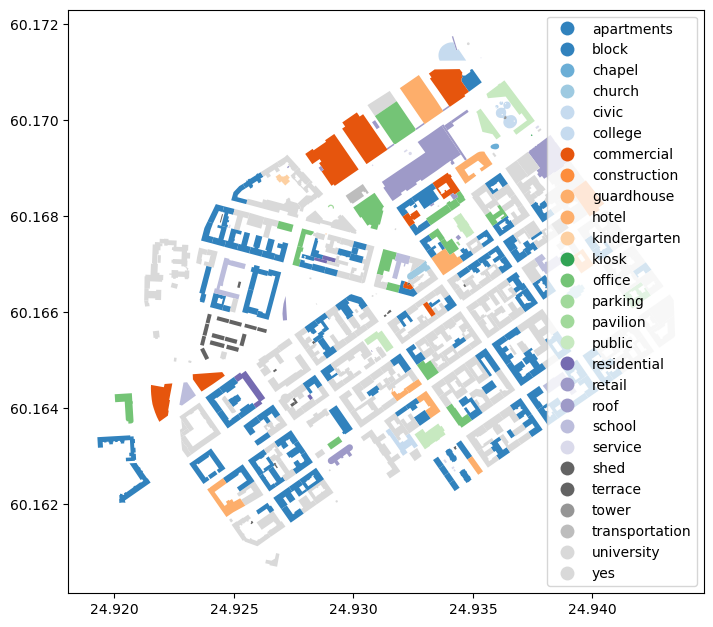
Figure 9.3. OSM buildings visualized by building tag values.
Let’s also fetch points of interests from our area of interest using the amenity tag:
tags = {"amenity": True}
amenities = ox.features.features_from_place(place, tags)
Again, let’s only plot a couple of available columns to check the contents of the data. You can see all column names by running list(amenities.columns).
amenities[["amenity", "name", "opening_hours", "geometry"]].head()
| amenity | name | opening_hours | geometry | ||
|---|---|---|---|---|---|
| element | id | ||||
| node | 60062502 | restaurant | Kabuki | NaN | POINT (24.92422 60.16725) |
| 60068035 | cafe | Cafe Java | Mo-Tu 09:00-21:00; We-Th 09:00-22:00; Fr 09:00... | POINT (24.93752 60.16997) | |
| 62965963 | restaurant | Restaurant & Bar Fusion | Mo-Th 11-22; Fr-Sa 11-02; Su 12-20 | POINT (24.93292 60.16953) | |
| 76617692 | restaurant | Johan Ludvig | NaN | POINT (24.92913 60.16781) | |
| 76624339 | restaurant | Shinobi | We-Th 17:00-23:00; Fr-Sa 16:00-24:00 | POINT (24.93194 60.16508) |
Here, we received all amenities in the area of interest ranging from restaurants, cafes and so on. The type of amenity (i.e., the value of the OSM tag) is indicated in the amenity column. Again, some, but not all features have additional information such as opening hours available. The downloaded data contains more than 700 individual points of interests in the data:
len(amenities)
757
Question 9.2#
How many different amenity categories are there?
Show code cell content
# Solution

# Get number of unique values in column `amenity`
amenities["amenity"].nunique()
63
Let’s limit our query to contain only restaurants and cafes in our area of interest. We can do this by specifying one or several tag values in the dictionary.
tags = {"amenity": ["restaurant", "cafe"]}
amenities = ox.features.features_from_place(place, tags)
len(amenities)
214
In addition to streets, buildings and amenities, OSM contains information about various land use features that can be useful for urban geospatial analysis. Let’s see how we can fetch urban green space data from OSM using the osmnx features module. Fetching green spaces from OpenStreetMap requires a bit of investigation of appropriate tag values and these might vary across cities.
One common way of tagging urban parks is leisure=park. If wanting to capture also other green infrastructure, additional tags such as landuse=grass may be added. Let’s proceed with these two tags that should capture most of the available greenspaces in downtown Helsinki.
# List key-value pairs for tags
tags = {"leisure": "park", "landuse": "grass"}
# Get the data
parks = ox.features.features_from_place(place, tags)
print("Retrieved", len(parks), "objects")
parks[["leisure", "landuse", "name", "geometry"]].head()
Retrieved 121 objects
| leisure | landuse | name | geometry | ||
|---|---|---|---|---|---|
| element | id | ||||
| relation | 9102643 | park | NaN | Ruoholahdenpuisto | MULTIPOLYGON (((24.91408 60.16148, 24.91408 60... |
| way | 8042256 | park | NaN | Pikkuparlamentinpuisto | POLYGON ((24.93566 60.17132, 24.93566 60.1713,... |
| 8042613 | park | NaN | Simonpuistikko | POLYGON ((24.93701 60.16947, 24.93627 60.16919... | |
| 15218362 | park | NaN | Työmiehenpuistikko | POLYGON ((24.9233 60.16499, 24.92323 60.165, 2... | |
| 15218739 | park | NaN | Lastenlehto | POLYGON ((24.92741 60.16575, 24.92741 60.16574... |
The first five rows of data contain different parks, which all have a name. Let’s quicly plot the data to see the geometry. By adding transparency to the map with the alpha parameter, we can observe where some of the grass and park polygon features overlap.
parks.plot(color="green", alpha=0.5)
<Axes: >
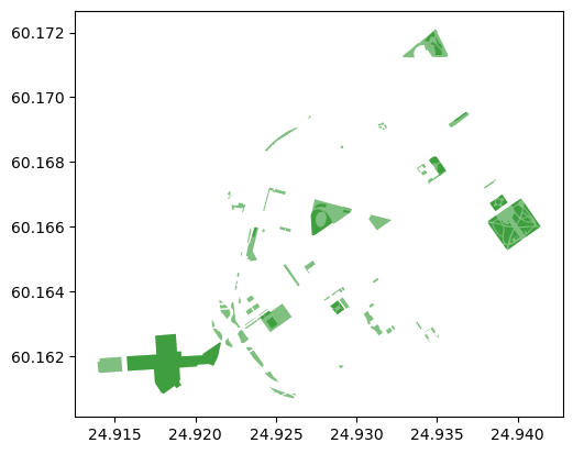
Figure 9.4. Polygons tagged with “leisure=park” or “landuse=grass”.
Plotting the data#
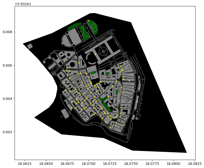
Let’s create a map that shows the data we downloaded.
import matplotlib.pyplot as plt

fig, ax = plt.subplots(figsize=(8.5, 8))

# Plot the footprint
aoi.plot(ax=ax, facecolor="black")

# Plot street edges
edges.plot(ax=ax, linewidth=1, edgecolor="dimgray")

# Plot buildings
buildings.plot(ax=ax, facecolor="silver", alpha=0.7)

parks.plot(ax=ax, facecolor="green", alpha=0.7)

# Plot restaurants
amenities.plot(ax=ax, color="yellow", alpha=0.7, markersize=10)

plt.tight_layout()
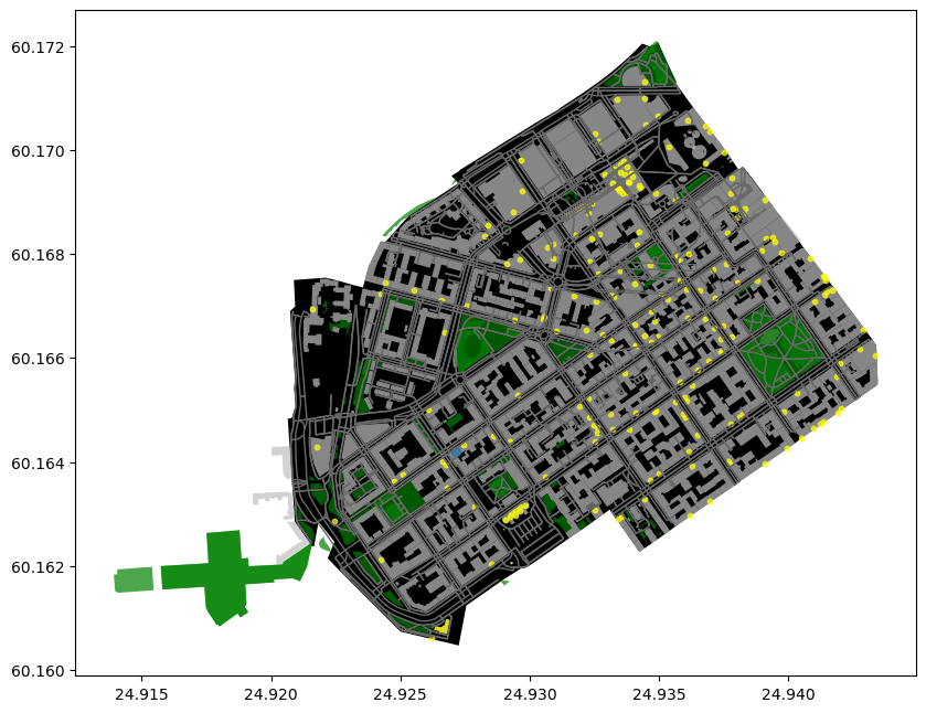
Figure 9.5. Visualization of OSM map features from the Kamppi area in Helsinki, Finland.
Alternative spatial queries#
If your area of interest is not represented by any existing featue in OSM, you can also query data based on custom polygon, bounding box or based on a buffer around a point or address location. Each way of querying the data is implemented in a distinct osmnx function. Here are the available fucntions for querying map features by:
address: osmnx.features.features_from_address(address, tags, dist)
bounding box: osmnx.features.features_from_bbox(bbox, tags)
point: osmnx.features.features_from_point(center_point, tags, dist)
polygon: osmnx.features.features_from_polygon(polygon, tags)
Similar alternative search functions exists for querying the network graph. See osmnx user reference for exact syntax.
Let’s try out querying data based on a pre-defined bounding box around the Cental railway station in Helsinki. Bounding box coordinates should be given in the correct order (left, bottom, right, top).
bounds = (24.9351773, 60.1641551, 24.9534055, 60.1791068)
buildings = ox.features.features_from_bbox(bounds, {"building": True})
buildings.plot()
<Axes: >
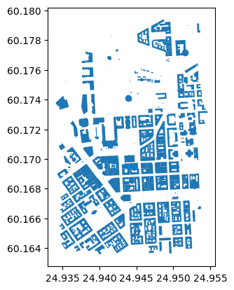
Figure 9.6. Downloaded buildings within a bounding box.
Here is another example of querying data within a distance treshold from a geocodable address. The distance parameter is given in meters.
address = "Central railway station, Helsinki, Finland"
tags = {"building": True}
distance = 500
buildings = ox.features.features_from_address(address, tags, distance)
buildings.plot()
<Axes: >
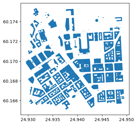
Figure 9.7. Downloaded buildings within a distance treshold from a geocoded address.
Question 9.3#
Check your understanding and retrieve OpenStreetMap data from some other area in the world. Use osmnx and download:
Polygon of your area of interest
Street network
Building footprints
Restaurants and cafes (or why not also other amenities)
Green spaces
Note that the larger the area you choose, the longer it takes to retrieve data from the API! When fetching the street network, you can use parameter network_type to limit the graph query to only specific types of roads.
Show code cell content
# Solution

# Example solution
place = "Gamla stan, Stockholm, Sweden"
aoi = ox.geocoder.geocode_to_gdf(place)

# Street network
graph = ox.graph.graph_from_place(place, network_type="walk")
edges = ox.convert.graph_to_gdfs(graph, nodes=False, edges=True)

# Other map features
buildings = ox.features.features_from_place(place, tags={"building": True})
amenities = ox.features.features_from_place(
    place, tags={"amenity": ["restaurant", "cafe"]}
)
parks = ox.features.features_from_place(
    place, tags={"leisure": "park", "landuse": "grass"}
)

# Plot the result
fig, ax = plt.subplots(figsize=(8.5, 8))

aoi.plot(ax=ax, facecolor="black")
edges.plot(ax=ax, linewidth=1, edgecolor="dimgray")
buildings.plot(ax=ax, facecolor="silver", alpha=0.7)
parks.plot(ax=ax, facecolor="green", alpha=0.7)
amenities.plot(ax=ax, color="yellow", alpha=0.7, markersize=10)
plt.tight_layout()